20 Linear model synthesis
We now have assembled all our tools for constructing and studying linear models. In this section, we summarize the tools we have acquired, and practice them in a variety of ways. Always, we are trying to understand our models from three perspectives:
- Data table,
- Equation,
- Plot.
20.1 General features of the linear model
Our linear model is based on two numbers:
- \(b\) is the base value,
- \(m\) is the rate.
We can interpret these two numbers in all three perspectives.
Data table.
The base \(b\) tells us \(\underline{\hspace{2in}}\).
The rate \(m\) tells us \(\underline{\hspace{2in}}\).
We can compute the rate from the table using \[ m = \frac{\qquad\qquad}{\qquad\qquad} \]
Equation.
The base and rate give us the equation \(\underline{\hspace{2in}}\).
Plot.
In terms of the plot, the base \(b\) gives us \(\underline{\hspace{2in}}\).
In terms of the plot, the rate \(m\) gives us \(\underline{\hspace{2in}}\).
Solutions
Data table. The base \(b\) is the starting value for \(y\), meaning the value of \(y\) when \(x = 0\).
The rate \(m\) tells us how much \(y\) changes for each unit increase in \(x\). The rate is computed as \(m = \dfrac{\text{change in } y}{\text{change in } x}\).
Equation. The base and rate give the equation \(y = b + mx\).
Plot. The base \(b\) is the \(y\)-intercept, where the line crosses the \(y\) axis. The rate \(m\) is the slope of the line.
20.2 Suppose we are given a scenario in words
We first want to check to determine whether or not a linear model is appropriate.
If a linear model is appropriate, then we can construct the data table, the equation, and the plot.
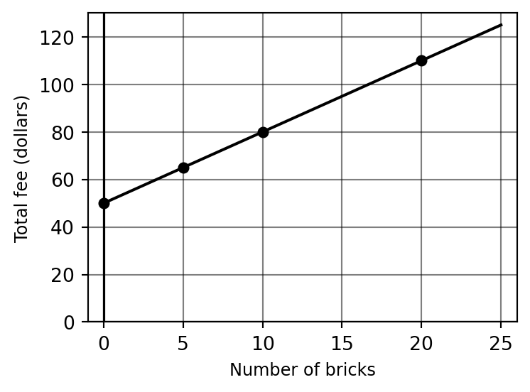
Example 20.1 (Activity: Scenario in words) The Taos Adobe Center charges $3 per adobe brick, plus a $50 packing fee.
- Explain why the relationship between \(x=\) the number of adobe bricks and \(y=\) the fee charged is linear.
- Construct a small data table for \(x\) and \(y\).
- Construct an equation relating \(x\) and \(y\).
- Make a plot of the linear relationship.
Solutions
The fee has two parts: a fixed packing fee ($50) and a per-brick charge ($3 each). Because the per-brick cost is constant, the total increases by the same amount for each additional brick. This is a constant rate of change, so a linear model is appropriate.
Let \(x\) = number of bricks, \(y\) = total fee (dollars).
| \(x\) | \(y\) |
|---|---|
| 0 | 50 |
| 5 | 65 |
| 10 | 80 |
| 20 | 110 |
\(y = 50 + 3x\)
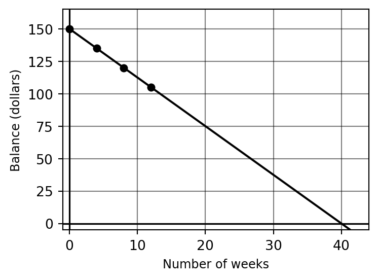
Example 20.2 (Activity: Scenario in words) Dr. Gutierrez is given a $150 certificate for the Taos Cow. She rewards herself with a scoop of Rio Grande Cherry Ristra each Friday afternoon, costing her $3.75 per week.
- Explain why the relationship between \(x=\) the number of weeks and \(y=\) the balance on her gift card is linear.
- Construct a small data table for \(x\) and \(y\).
- Construct an equation relating \(x\) and \(y\).
- Make a plot of the linear relationship.
Solutions
The balance decreases by the same amount ($3.75) each week. This is a constant rate of change, so a linear model is appropriate.
Let \(x\) = number of weeks, \(y\) = balance (dollars).
| \(x\) | \(y\) |
|---|---|
| 0 | 150 |
| 4 | 135 |
| 8 | 120 |
| 12 | 105 |
\(y = 150 - 3.75x\)
20.3 Suppose we are given the plot
If we are given the plot of a linear model, we can construct a data table and also construct the equation.
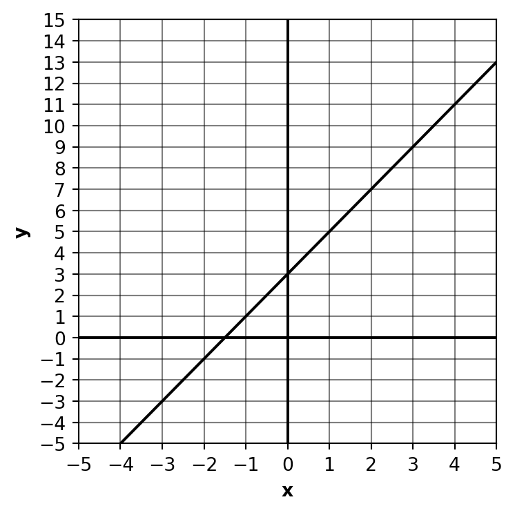
Example 20.3 (Activity: Given the plot) Construct a small data table and find the equation of the line.
Solutions
The line crosses the \(y\) axis at \(3\), so \(b = 3\). For each unit increase in \(x\), \(y\) increases by \(2\), so \(m = 2\).
| \(x\) | \(y\) |
|---|---|
| 0 | 3 |
| 1 | 5 |
| 2 | 7 |
| 3 | 9 |
Equation: \(y = 3 + 2x\).
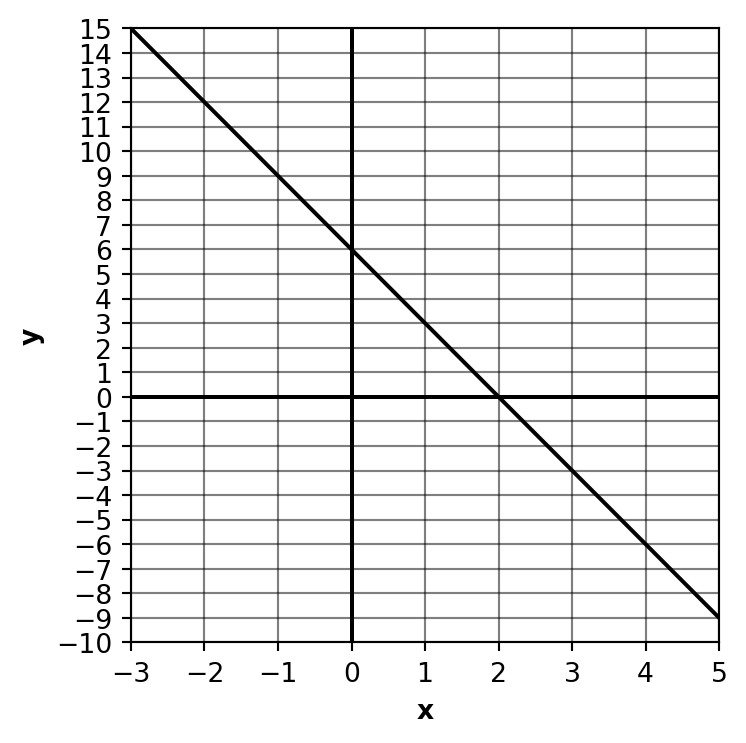
Example 20.4 (Activity: Given the plot) Construct a small data table and find the equation of the line.
Solutions
The line crosses the \(y\) axis at \(6\), so \(b = 6\). For each unit increase in \(x\), \(y\) decreases by \(3\), so \(m = -3\).
| \(x\) | \(y\) |
|---|---|
| 0 | 6 |
| 1 | 3 |
| 2 | 0 |
| 3 | -3 |
Equation: \(y = 6 - 3x\).
20.4 Suppose we are given an equation
If we are given the equation for a linear model, we can construct a data table and also construct the plot.
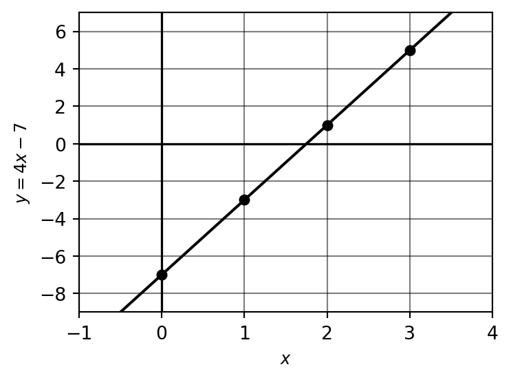
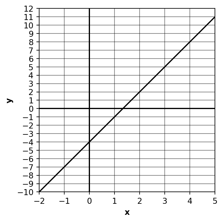
Example 20.5 (Activity: Given the equation) Consider the equation \(y = 4x - 7\). Construct a small data table, and then sketch the plot of the line.
Solutions
| \(x\) | \(y\) |
|---|---|
| 0 | -7 |
| 1 | -3 |
| 2 | 1 |
| 3 | 5 |
Base \(b = -7\), slope \(m = 4\).
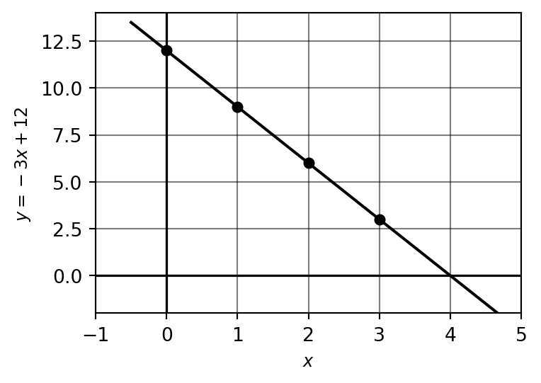
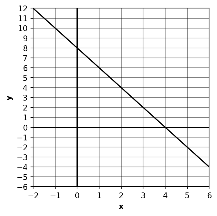
Example 20.6 (Activity: Given the equation) Consider the equation \(y = -3x + 12\). Construct a small data table, and then sketch the plot of the line.
Solutions
| \(x\) | \(y\) |
|---|---|
| 0 | 12 |
| 1 | 9 |
| 2 | 6 |
| 3 | 3 |
Base \(b = 12\), slope \(m = -3\).
20.5 Suppose we are given a data table
If we are given a data table for a linear model, we can construct the equation and we can construct the plot.
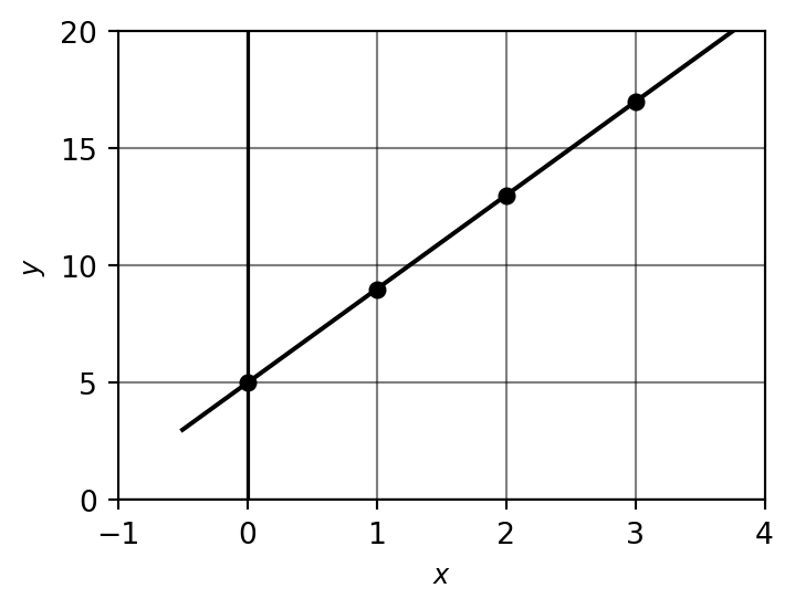
Example 20.7 (Activity: Given the data table) Here is a data table. Construct the equation for the linear model that matches the table, and sketch the plot.
| \(x\) | \(y\) |
|---|---|
| 0 | 5 |
| 1 | 9 |
| 2 | 13 |
| 3 | 17 |
Solutions
Rate: \(m = \dfrac{9 - 5}{1 - 0} = 4\). Base: \(b = 5\) (the value at \(x = 0\)).
Equation: \(y = 5 + 4x\).
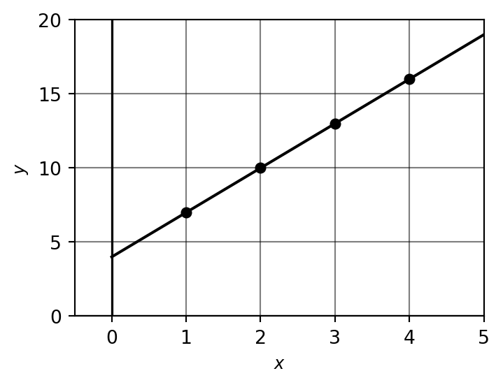
Example 20.8 (Activity: Given the data table) Here is a data table. Construct the equation for the linear model that matches the table, and sketch the plot.
| \(x\) | \(y\) |
|---|---|
| 1 | 7 |
| 2 | 10 |
| 3 | 13 |
| 4 | 16 |
Solutions
Rate: \(m = \dfrac{10 - 7}{2 - 1} = 3\). Base: using \((1, 7)\): \(7 = b + 3 \cdot 1 \Rightarrow b = 4\).
Equation: \(y = 4 + 3x\).
Sometimes the data takes the form of given points on a graphic, rather than a formal data table.
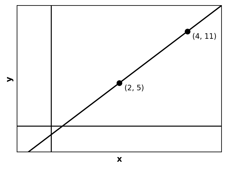
Example 20.9 (Activity: Given the plot (no grid)) Find the equation of the line in the plot below. Then find the point where the line crosses the \(x\) axis.
Solutions
Slope: \(m = \dfrac{11 - 5}{4 - 2} = \dfrac{6}{2} = 3\). Base: \(5 = b + 3 \cdot 2 \Rightarrow b = -1\).
Equation: \(y = -1 + 3x\).
\(x\)-intercept: \(0 = -1 + 3x \Rightarrow x = \dfrac{1}{3}\). The line crosses the \(x\) axis at \(\left(\dfrac{1}{3}, 0\right)\).
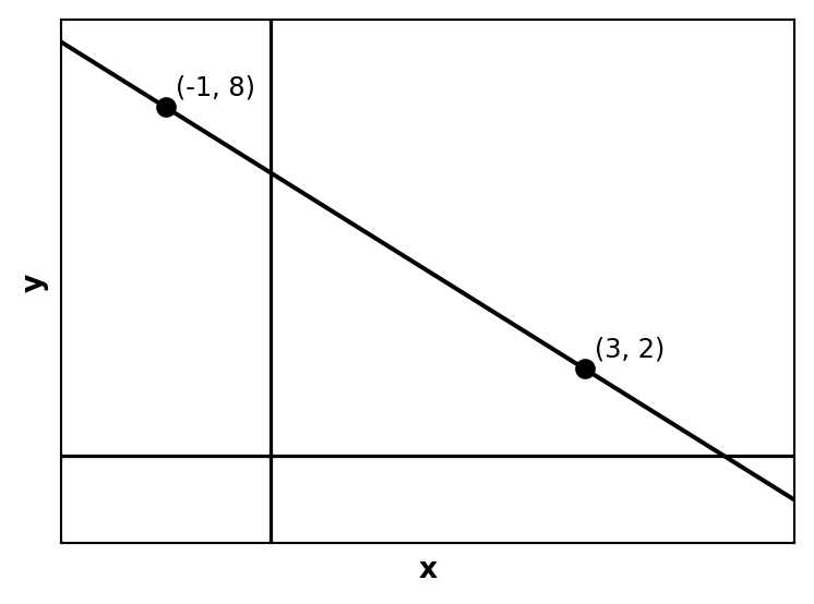
Example 20.10 (Activity: Given the plot (no grid)) Find the equation of the line in the plot below. Then find the point where the line crosses the \(x\) axis.
Solutions
Slope: \(m = \dfrac{2 - 8}{3 - (-1)} = \dfrac{-6}{4} = -\dfrac{3}{2}\). Base: \(8 = b + \left(-\dfrac{3}{2}\right)(-1) \Rightarrow b = 8 - \dfrac{3}{2} = \dfrac{13}{2}\).
Equation: \(y = \dfrac{13}{2} - \dfrac{3}{2}x\).
\(x\)-intercept: \(0 = \dfrac{13}{2} - \dfrac{3}{2}x \Rightarrow x = \dfrac{13}{3}\). The line crosses the \(x\) axis at \(\left(\dfrac{13}{3}, 0\right)\).
20.6 Homework exercises
Exercise 20.1 Make a data table, and find the equation, for the following line.
Solutions
The line crosses the \(y\) axis at \(8\), so \(b = 8\). The line falls \(2\) units for each unit right, so \(m = -2\).
| \(x\) | \(y\) |
|---|---|
| 0 | 8 |
| 1 | 6 |
| 2 | 4 |
| 3 | 2 |
Equation: \(y = 8 - 2x\).
Exercise 20.2 Make a data table, and find the equation, for the following line.
Solutions
The line crosses the \(y\) axis at \(-4\), so \(b = -4\). The line rises \(3\) units for each unit right, so \(m = 3\).
| \(x\) | \(y\) |
|---|---|
| 0 | -4 |
| 1 | -1 |
| 2 | 2 |
| 3 | 5 |
Equation: \(y = -4 + 3x\).
Exercise 20.3 Consider the equation \(y = 6x + 2\). Construct a small data table, and then sketch the plot of the line.
Solutions
| \(x\) | \(y\) |
|---|---|
| 0 | 2 |
| 1 | 8 |
| 2 | 14 |
| 3 | 20 |
Base \(b = 2\), slope \(m = 6\).
Exercise 20.4 Consider the equation \(y = 18 - 3x\). Construct a small data table, and then sketch the plot of the line.
Solutions
| \(x\) | \(y\) |
|---|---|
| 0 | 18 |
| 1 | 15 |
| 2 | 12 |
| 3 | 9 |
Base \(b = 18\), slope \(m = -3\).
Exercise 20.5 Here is a data table. Construct the equation for the linear model that matches the table, and sketch the plot.
| \(x\) | \(y\) |
|---|---|
| 2 | 11 |
| 3 | 14 |
| 4 | 17 |
| 5 | 20 |
Solutions
Rate: \(m = \dfrac{14 - 11}{3 - 2} = 3\). Base: \(11 = b + 3 \cdot 2 \Rightarrow b = 5\).
Equation: \(y = 5 + 3x\).
Exercise 20.6 Here is a data table. Construct the equation for the linear model that matches the table, and sketch the plot.
| \(x\) | \(y\) |
|---|---|
| 1 | 12 |
| 2 | 9 |
| 3 | 6 |
| 4 | 3 |
Solutions
Rate: \(m = \dfrac{9 - 12}{2 - 1} = -3\). Base: \(12 = b + (-3) \cdot 1 \Rightarrow b = 15\).
Equation: \(y = 15 - 3x\).
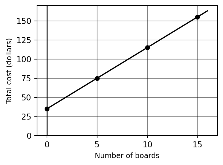
Exercise 20.7 The Taos Lumber Yard charges $8 per board of pine wood, plus a $35 delivery fee.
- Explain why the relationship between \(x=\) the number of boards and \(y=\) the total cost is linear.
- Construct a small data table for \(x\) and \(y\).
- Construct an equation relating \(x\) and \(y\).
- Make a plot of the linear relationship.
Solutions
The total cost has a fixed delivery fee ($35) plus a constant per-board cost ($8). The constant rate of change makes a linear model appropriate.
Let \(x\) = number of boards, \(y\) = total cost (dollars).
| \(x\) | \(y\) |
|---|---|
| 0 | 35 |
| 5 | 75 |
| 10 | 115 |
| 15 | 155 |
\(y = 35 + 8x\)
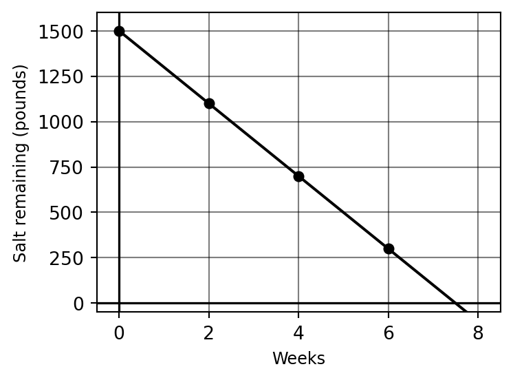
Exercise 20.8 At the beginning of the winter, the Taos County Road Division orders 1500 pounds of salt for treating roads. They estimate that they will use, on average, 200 pounds of salt per week.
- Explain why the relationship between \(x=\) the number of weeks of winter and \(y=\) the amount of salt remaining is linear.
- Construct a small data table for \(x\) and \(y\).
- Construct an equation relating \(x\) and \(y\).
- Make a plot of the linear relationship.
Solutions
The salt decreases by a constant 200 pounds per week. This constant rate of change makes a linear model appropriate.
Let \(x\) = number of weeks, \(y\) = salt remaining (pounds).
| \(x\) | \(y\) |
|---|---|
| 0 | 1500 |
| 2 | 1100 |
| 4 | 700 |
| 6 | 300 |
\(y = 1500 - 200x\)
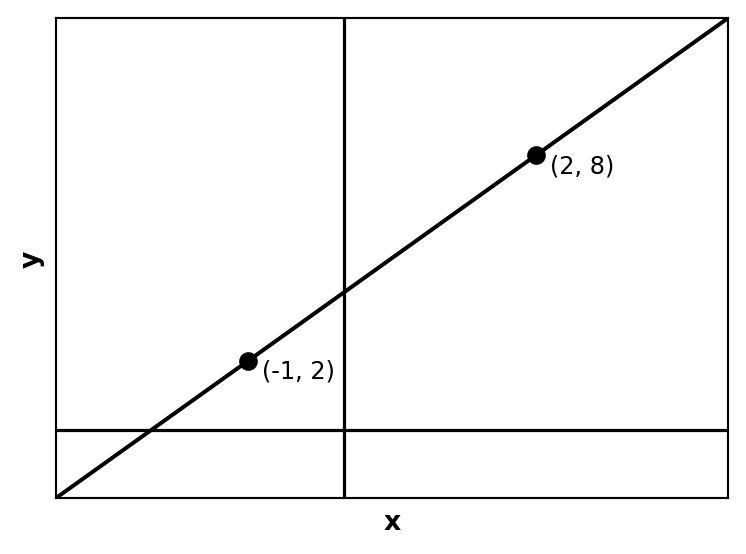
Exercise 20.9 Find the equation of the line in the plot below. Then find the point where the line crosses the \(x\) axis.
Solutions
Slope: \(m = \dfrac{8 - 2}{2 - (-1)} = \dfrac{6}{3} = 2\). Base: \(2 = b + 2 \cdot (-1) \Rightarrow b = 4\).
Equation: \(y = 4 + 2x\).
\(x\)-intercept: \(0 = 4 + 2x \Rightarrow x = -2\). The line crosses the \(x\) axis at \((-2, 0)\).
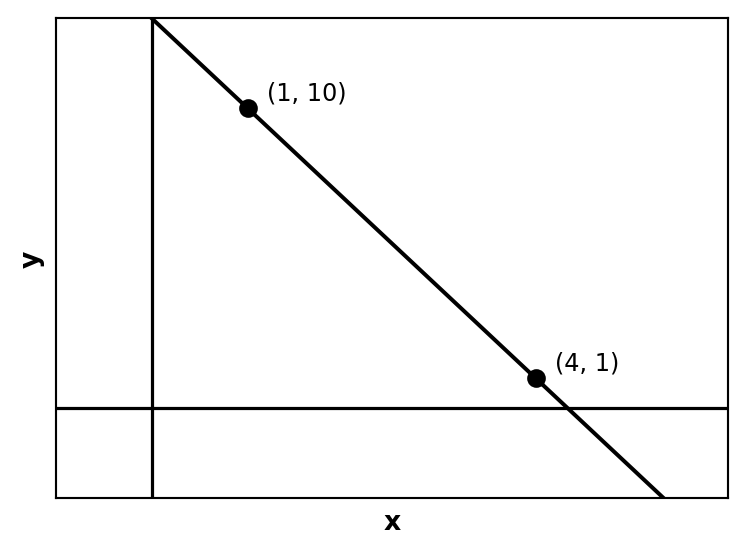
Exercise 20.10 Find the equation of the line in the plot below. Then find the point where the line crosses the \(x\) axis.
Solutions
Slope: \(m = \dfrac{1 - 10}{4 - 1} = \dfrac{-9}{3} = -3\). Base: \(10 = b + (-3) \cdot 1 \Rightarrow b = 13\).
Equation: \(y = 13 - 3x\).
\(x\)-intercept: \(0 = 13 - 3x \Rightarrow x = \dfrac{13}{3}\). The line crosses the \(x\) axis at \(\left(\dfrac{13}{3}, 0\right)\).