25 Exponential models with percent change
In this section we analyze exponential models related to percent increase and decrease.
Example 25.1 (Activity: Fruit fly population) Due to an abandoned pile of bananas, fruit flies are growing rapidly in the kitchen. At the start of the week, there are 3 fruit flies. The number of fruit flies increases at a rate of 200% per day.
Increasing by 200% per day means that each day the population is \(100\% + 200\% = 300\%\) of the previous day’s population.
This means that after 1 day, the number of fruit flies is \[ \text{Flies Day 1} = \text{300\% of } 3 = \underline{\hspace{2in}} \]
Use this information to complete the following data table.
| Day | Fruit Flies |
|---|---|
| \(\phantom{\dfrac{1}{2}}\) 0 | 3 |
| \(\phantom{\dfrac{1}{2}}\) 1 | |
| \(\phantom{\dfrac{1}{2}}\) 2 | |
| \(\phantom{\dfrac{1}{2}}\) 3 |
What number do we multiply the fly population by to get the next day’s population?
Using the variables
- \(x\) is the number of days,
- \(y\) is the number of flies,
construct a formula for the number of flies each day.
In terms of the standard formula \(y = A \cdot R^x\):
- What is the value of \(A\)?
- What is the value of \(R\)?
How many flies does the model predict will be in the kitchen after 1 week?
Solutions
| Day | Fruit Flies |
|---|---|
| 0 | 3 |
| 1 | 9 |
| 2 | 27 |
| 3 | 81 |
The population is multiplied by \(R = 3\) each day (since \(300\% = 3\)).
\(A = 3\) (initial population), \(R = 3\).
Formula: \(y = 3 \cdot 3^x\).
After 1 week (\(x = 7\)): \(y = 3 \cdot 3^7 = 3 \cdot 2187 = 6{,}561\) flies.
25.1 The percent change framework
When a quantity changes by a fixed percent each time period, the multiplier \(R\) is determined by the percent rate \(r\):
- If the quantity increases by \(r\) each period, then \(R = 1 + r\).
- If the quantity decreases by \(r\) each period, then \(R = 1 - r\).
The formula is then \[ y = A \cdot R^x, \] where \(A\) is the starting amount and \(x\) is the number of time periods.
Example 25.2 (Activity: Fishing guides wage increase) The Association of Taos County Fishing Guides has negotiated a new contract. Currently, fishing guides are paid $20 per hour. Under their contract, this amount will increase by 5% each year for the next 6 years. We want to model the hourly wage during the duration of the contract.
What is the starting amount \(A\) in this situation?
What is the rate \(r\)? What are the time units?
What is the multiplier \(R = 1 + r\)?
Using the variables \(x =\) years and \(y =\) hourly wage (dollars), write the equation for this model. \[ y = \underline{\hspace{3in}} \]
What will the guides’ hourly wage be after 6 years?
Solutions
\(A = \$20\) per hour.
\(r = 0.05\) (5% annual increase), time units are years.
\(R = 1 + 0.05 = 1.05\).
Formula: \(y = 20 \cdot (1.05)^x\).
After 6 years: \(y = 20 \cdot (1.05)^6 \approx 20 \cdot 1.3401 \approx \$26.80\) per hour.
25.2 Practice
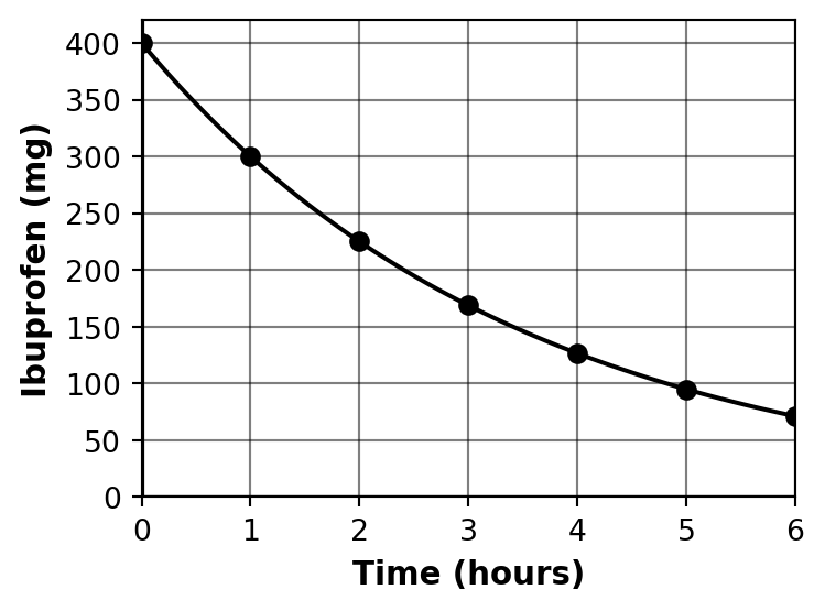
Example 25.3 (Activity: Ibuprofen metabolism) A patient takes a 400 mg pill of ibuprofen. The following plot shows the amount of drug available to the body, which decreases as the drug is metabolized. Use the plot to identify \(A\) and \(R\), and construct a formula for the amount of available ibuprofen (mg) in terms of time (hours). Use the value of \(R\) to determine the percent decrease per hour.
Solutions
Reading from the plot: at \(x = 0\) the amount is 400 mg, so \(A = 400\).
The ratio between consecutive values: \(\dfrac{300}{400} = 0.75\), so \(R = 0.75\).
In terms of the percent framework: each hour 25% is metabolized, so \(r = 0.25\) and \(R = 1 - r = 0.75\).
Formula: \(y = 400 \cdot (0.75)^x\).
Since \(R=0.75 = 1-0.25\), there is a 25% decrease per hour.
Example 25.4 (Activity: Mora County population) The 2020 population of Mora County was 4,189. Suppose that the county grows at 3% per year for the following decade.
- Make a data table for the population over time.
- Construct a formula for the population in terms of years since 2020.
- Sketch a plot of your model.
- According to your model, what will the population be in 2030? Label this point on your plot.
Solutions
\(A = 4189\), \(r = 0.03\), \(R = 1.03\), \(x =\) years since 2020, \(y =\) population.
| Year (\(x\)) | Population (\(y\)) |
|---|---|
| 0 | 4,189 |
| 1 | 4,315 |
| 2 | 4,444 |
| 3 | 4,577 |
| 4 | 4,715 |
| 5 | 4,856 |
Formula: \(y = 4189 \cdot (1.03)^x\).
2030 population (\(x = 10\)): \(y = 4189 \cdot (1.03)^{10} \approx 4189 \cdot 1.3439 \approx 5{,}630\).
Example 25.5 (Activity: Truck depreciation) The value of equipment decreases over time; this is called depreciation. It is typical for pickup trucks to depreciate in such a way that they lose 10% of their value each year. Consider a new truck that costs $50,000.
- Make a data table showing the value of the truck over a five year period.
- Construct a formula for the value of the truck over time.
- Sketch a plot of the value over time.
- What does your model predict the value will be 10 years after purchase? Label this point on your plot.
Solutions
\(A = 50000\), \(r = 0.10\) (depreciation rate), \(R = 1 - 0.10 = 0.90\), \(x =\) years, \(y =\) value (dollars).
| Year (\(x\)) | Value (\(y\)) |
|---|---|
| 0 | $50,000.00 |
| 1 | $45,000.00 |
| 2 | $40,500.00 |
| 3 | $36,450.00 |
| 4 | $32,805.00 |
| 5 | $29,524.50 |
Formula: \(y = 50000 \cdot (0.90)^x\).
After 10 years: \(y = 50000 \cdot (0.90)^{10} \approx 50000 \cdot 0.3487 \approx \$17{,}434\).
25.3 Homework exercises
Exercise 25.1 $2,000 is put into a savings account that earns 4% interest per year, compounded annually.
- Construct a data table showing the value of the account each year for 5 years.
- Make a plot showing the data in your table.
- Write down the formula for the value in terms of years.
- How much money will be in the account after 5 years?
Solutions
\(A = 2000\), \(r = 0.04\), \(R = 1.04\), \(x =\) years.
| Year (\(x\)) | Value (\(y\)) |
|---|---|
| 0 | $2,000.00 |
| 1 | $2,080.00 |
| 2 | $2,163.20 |
| 3 | $2,249.73 |
| 4 | $2,339.72 |
| 5 | $2,433.31 |
Formula: \(y = 2000 \cdot (1.04)^x\).
After 5 years: \(y \approx \$2{,}433.31\).
Exercise 25.2 A patient takes 500 mg of a medication. Each hour, 15% of the medication is eliminated from the bloodstream.
- Construct a data table showing the amount of medication in the patient each hour.
- Make a plot showing the data in your table.
- Write down the formula for the medication in terms of hours.
- How much medication remains after 6 hours?
Solutions
\(A = 500\), \(r = 0.15\) (elimination rate per hour), \(R = 1 - 0.15 = 0.85\), \(x =\) hours.
| Hour (\(x\)) | Medication (\(y\), mg) |
|---|---|
| 0 | 500.00 |
| 1 | 425.00 |
| 2 | 361.25 |
| 3 | 307.06 |
| 4 | 261.00 |
| 5 | 221.85 |
| 6 | 188.57 |
Formula: \(y = 500 \cdot (0.85)^x\).
After 6 hours: \(y = 500 \cdot (0.85)^6 \approx 188.6\) mg.
Exercise 25.3 Consider the exponential model \[ y = 500 \cdot 2.5^x, \] where \(x\) is measured in years.
- What is the starting amount \(A\) for this model?
- What is \(R\)? What is the annual percent growth rate \(r\)?
- Draw a sketch of the plot for this model.
- What will the amount be after 7 years? Show this point on your plot.
Solutions
\(A = 500\).
\(R = 2.5\). Since \(R = 1 + r\), we get \(r = R - 1 = 1.5\), i.e., a 150% annual growth rate.
After 7 years: \(y = 500 \cdot 2.5^7 \approx 500 \cdot 610.4 \approx \$305{,}176\).
Exercise 25.4 A small town currently has a population of 1,000 residents. Two analysts make different projections for the town’s growth over the next decade.
- Analyst A projects that the population will grow by 100 residents per year.
- Analyst B projects that the population will grow by 10% per year.
- Make a data table for each projection, showing the population for the first 6 years.
- Write a formula for each projection. Use \(x =\) years and \(y =\) population.
- Both projections give the same population after 1 year. Explain why this makes sense.
- Which projection predicts a larger population after 10 years? By how much?
Solutions
Analyst A (linear): The population increases by a constant 100 each year. Formula: \(y = 1000 + 100x\).
Analyst B (exponential): \(A = 1000\), \(r = 0.10\), \(R = 1.10\). Formula: \(y = 1000 \cdot (1.10)^x\).
| Year (\(x\)) | Analyst A | Analyst B |
|---|---|---|
| 0 | 1,000 | 1,000 |
| 1 | 1,100 | 1,100 |
| 2 | 1,200 | 1,210 |
| 3 | 1,300 | 1,331 |
| 4 | 1,400 | 1,464 |
| 5 | 1,500 | 1,611 |
| 6 | 1,600 | 1,772 |
Both give 1,100 after year 1 because 10% of the starting population of 1,000 is exactly 100 — the same as the linear rate.
After 10 years: Analyst A gives \(1000 + 100 \cdot 10 = 2{,}000\). Analyst B gives \(1000 \cdot (1.10)^{10} \approx 1000 \cdot 2.594 \approx 2{,}594\). The exponential projection predicts about 594 more residents.