19 The concept of slope
The goal for this section is to better understand the rate part of linear models. We want to gain a geometric understanding of the rate, as well as learn how to compute the rate from a data table. We begin with two motivating examples.
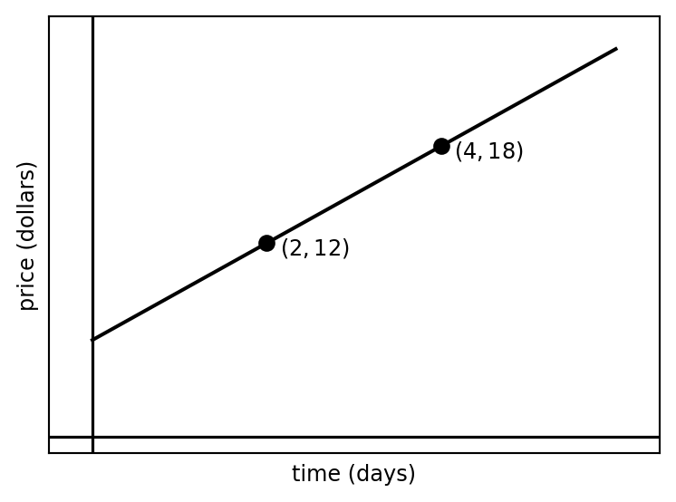
Example 19.1 Jim is running a private parking lot near the Alamosa Airport. He charges $12 for 2 days. He charges $18 for 4 days. We are going to assume that we have a linear relation between days and price.
- First we the plot for this scenario, with time on the horizontal axis and price on the vertical axis. Put the two data points on the sketch.
- What are the units of the rate?
- Compute the rate, writing it as a fraction.
Example 19.2 Martin is driving to Denver. After 2 hours, he has traveled 100 miles. After 4 hours, he has traveled 210 miles.
- Sketch the plot for this scenario, with time on the horizontal axis and distance on the vertical axis. Put the two data points on the sketch.
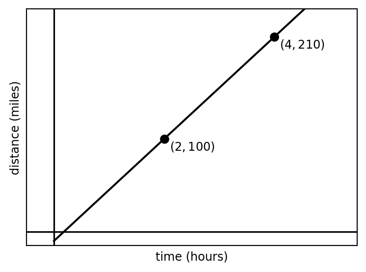
- What are the units of the rate?
- Compute the rate, writing it as a fraction.
19.1 General formula for rate
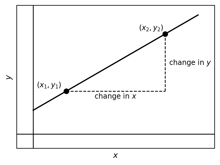
With \(x\) as the horizontal (input) variable and \(y\) as the vertical (output) variable, we can compute the rate as follows:
\[ \text{rate} = \frac{\text{change in } y}{\text{change in } x} \]
19.2 Computing the rate from the plot
Compute the rate for each of the following lines.
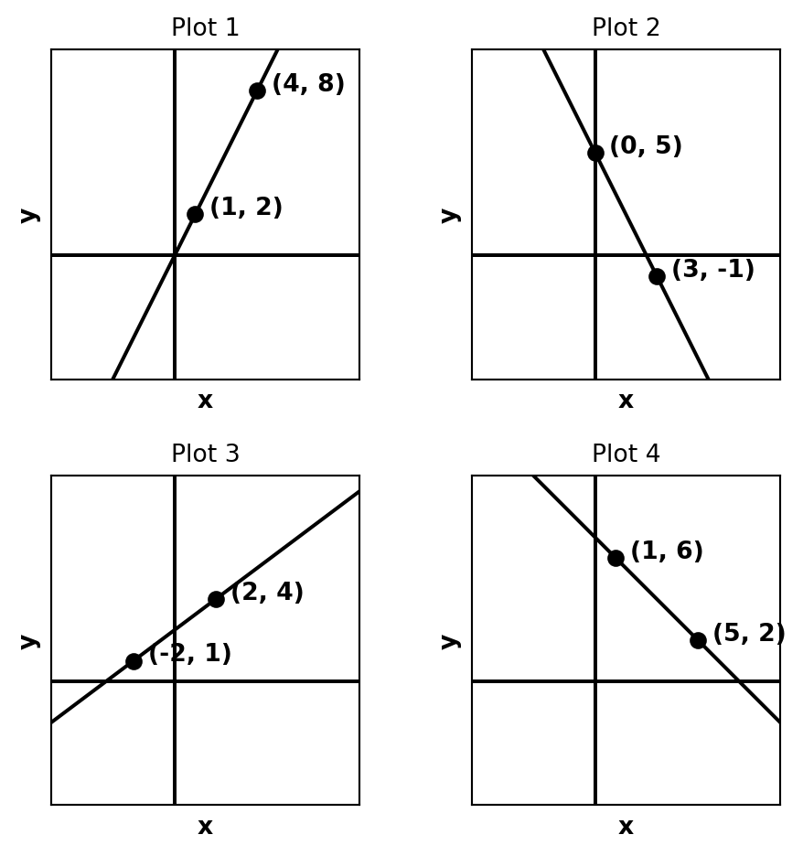
Discussion:
- For which plots is the rate positive? For those plots, which rate is larger?
- For which plots is the rate negative? For those plots, which rate is a larger negative value?
- The rate is also called the slope of the line. Why does this word make sense?
Solutions
Plots 1 and 3 have positive rates: Plot 1 has slope \(\dfrac{8-2}{4-1} = 2\) and Plot 3 has slope \(\dfrac{4-1}{2-(-2)} = \dfrac{3}{4}\). Plot 1 has the larger rate.
Plots 2 and 4 have negative rates: Plot 2 has slope \(\dfrac{-1-5}{3-0} = -2\) and Plot 4 has slope \(\dfrac{2-6}{5-1} = -1\). Plot 2 has the larger negative value (it is more negative).
“Slope” refers to the steepness of a line. A line with a large positive rate rises steeply as we move from left to right; a line with a large negative rate falls steeply. The word captures the geometric idea of how much the line tilts.
19.3 Computing slope from a data table
Example 19.3 (Activity: Computing slope from a data table) Use the two points in the data table to compute the slope. Then sketch the line.
| \(x\) | \(y\) |
|---|---|
| 2 | 7 |
| 5 | 16 |
Solutions
Slope: \(m = \dfrac{16 - 7}{5 - 2} = \dfrac{9}{3} = 3\).
Example 19.4 (Activity: Computing slope from a data table) Use the two points in the data table to compute the slope. Then sketch the line.
| \(x\) | \(y\) |
|---|---|
| 0 | 10 |
| 4 | 2 |
Solutions
Slope: \(m = \dfrac{2 - 10}{4 - 0} = \dfrac{-8}{4} = -2\).
Example 19.5 (Activity: Computing slope from a data table) Use the two points in the data table to compute the slope. Then sketch the line.
| \(x\) | \(y\) |
|---|---|
| -3 | 1 |
| 2 | 11 |
Solutions
Slope: \(m = \dfrac{11 - 1}{2 - (-3)} = \dfrac{10}{5} = 2\).
Example 19.6 (Activity: Computing slope from a data table) Use the two points in the data table to compute the slope. Then sketch the line.
| \(x\) | \(y\) |
|---|---|
| 1 | -2 |
| 6 | -12 |
Solutions
Slope: \(m = \dfrac{-12 - (-2)}{6 - 1} = \dfrac{-10}{5} = -2\).
19.4 Discussion: We have the slope, what about the base?
In the previous examples, we were able to compute the slope from the two data points. How can we use the data to compute the value of the base \(b\)?
Example 19.7 (Activity: Finding the equation from two points) Find the equation of the line having the points \((3,5)\) and \((8, 20)\).
Solutions
Slope: \(m = \dfrac{20 - 5}{8 - 3} = \dfrac{15}{5} = 3\).
Base: using the point \((3, 5)\): \(5 = b + 3 \cdot 3 \Rightarrow b = 5 - 9 = -4\).
Equation: \(y = -4 + 3x\).
Example 19.8 (Activity: Finding the equation from two points) Find the equation of the line having the points \((1,13)\) and \((4, 5)\).
Solutions
Slope: \(m = \dfrac{5 - 13}{4 - 1} = \dfrac{-8}{3}\).
Base: using the point \((1, 13)\): \(13 = b + \dfrac{-8}{3} \cdot 1 \Rightarrow b = 13 + \dfrac{8}{3} = \dfrac{47}{3}\).
Equation: \(y = \dfrac{47}{3} - \dfrac{8}{3}x\).
19.5 Section 19.3 revisited
Example 19.9 (Activity: Finding the base) In Example 19.3 you found the slope of the line passing through the data table. Now compute the value of the base \(b\) to get a complete linear equation.
Solutions
Using the point \((2, 7)\) and slope \(m = 3\): \(7 = b + 3 \cdot 2 \Rightarrow b = 7 - 6 = 1\).
Equation: \(y = 1 + 3x\).
Example 19.10 (Activity: Finding the base) In Example 19.4 you found the slope of the line passing through the data table. Now compute the value of the base \(b\) to get a complete linear equation.
Solutions
Using the point \((0, 10)\) and slope \(m = -2\): \(10 = b + (-2) \cdot 0 \Rightarrow b = 10\).
Equation: \(y = 10 - 2x\).
Example 19.11 (Activity: Finding the base) In Example 19.5 you found the slope of the line passing through the data table. Now compute the value of the base \(b\) to get a complete linear equation.
Solutions
Using the point \((-3, 1)\) and slope \(m = 2\): \(1 = b + 2 \cdot (-3) \Rightarrow b = 1 + 6 = 7\).
Equation: \(y = 7 + 2x\).
Example 19.12 (Activity: Finding the base) In Example 19.6 you found the slope of the line passing through the data table. Now compute the value of the base \(b\) to get a complete linear equation.
Solutions
Using the point \((1, -2)\) and slope \(m = -2\): \(-2 = b + (-2) \cdot 1 \Rightarrow b = -2 + 2 = 0\).
Equation: \(y = -2x\).
19.6 Homework exercises
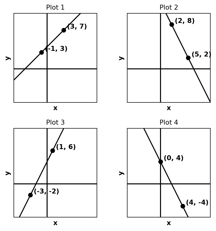
Exercise 19.1 For each plot below, compute the slope. Then find the equation of the line.
Solutions
Plot 1 \((-1, 3)\) and \((3, 7)\): slope \(= \dfrac{7-3}{3-(-1)} = 1\); base: \(3 = (-1)(1) + b \Rightarrow b = 4\). Equation: \(y = 4 + x\).
Plot 2 \((2, 8)\) and \((5, 2)\): slope \(= \dfrac{2-8}{5-2} = -2\); base: \(8 = 2(-2) + b \Rightarrow b = 12\). Equation: \(y = 12 - 2x\).
Plot 3 \((-3, -2)\) and \((1, 6)\): slope \(= \dfrac{6-(-2)}{1-(-3)} = 2\); base: \(-2 = (-3)(2) + b \Rightarrow b = 4\). Equation: \(y = 4 + 2x\).
Plot 4 \((0, 4)\) and \((4, -4)\): slope \(= \dfrac{-4-4}{4-0} = -2\); base: \(4 = 0(-2) + b \Rightarrow b = 4\). Equation: \(y = 4 - 2x\).
Exercise 19.2 For each pair of points, find the equation of the line. Then draw a sketch of the line. Finally, determine the point where the line crosses the \(x\) axis.
- \((1, 5)\) and \((3, 9)\)
- \((0, 4)\) and \((2, 0)\)
- \((-2, 1)\) and \((2, 5)\)
- \((1, 6)\) and \((4, 0)\)
- \((-1, -3)\) and \((3, 5)\)
- \((2, 8)\) and \((5, -1)\)
Solutions
\((1,5)\) and \((3,9)\): slope \(= \dfrac{9-5}{3-1} = 2\); base: \(5 = 2(1) + b \Rightarrow b = 3\). Equation: \(y = 3 + 2x\). \(x\)-intercept: \(0 = 3 + 2x \Rightarrow x = -\dfrac{3}{2}\).
\((0,4)\) and \((2,0)\): slope \(= \dfrac{0-4}{2-0} = -2\); base: \(b = 4\). Equation: \(y = 4 - 2x\). \(x\)-intercept: \(0 = 4 - 2x \Rightarrow x = 2\).
\((-2,1)\) and \((2,5)\): slope \(= \dfrac{5-1}{2-(-2)} = 1\); base: \(1 = (-2)(1) + b \Rightarrow b = 3\). Equation: \(y = 3 + x\). \(x\)-intercept: \(0 = 3 + x \Rightarrow x = -3\).
\((1,6)\) and \((4,0)\): slope \(= \dfrac{0-6}{4-1} = -2\); base: \(6 = (1)(-2) + b \Rightarrow b = 8\). Equation: \(y = 8 - 2x\). \(x\)-intercept: \(0 = 8 - 2x \Rightarrow x = 4\).
\((-1,-3)\) and \((3,5)\): slope \(= \dfrac{5-(-3)}{3-(-1)} = 2\); base: \(-3 = (-1)(2) + b \Rightarrow b = -1\). Equation: \(y = -1 + 2x\). \(x\)-intercept: \(0 = -1 + 2x \Rightarrow x = \dfrac{1}{2}\).
\((2,8)\) and \((5,-1)\): slope \(= \dfrac{-1-8}{5-2} = -3\); base: \(8 = (2)(-3) + b \Rightarrow b = 14\). Equation: \(y = 14 - 3x\). \(x\)-intercept: \(0 = 14 - 3x \Rightarrow x = \dfrac{14}{3}\).
Exercise 19.3 At Paul’s Tea Attic, customers pay a cover charge and also pay per drink.
- Graig orders one drink and is charged a total of $13.
- Maig orders four drinks and is charged a total of $28.
- Determine the per-drink cost and also the cover charge.
- Make a data table showing the total cost for up to drinks.
- Make a plot showing cost on the vertical axis and number of drinks on the horizontal axis.
- How many cups of tea can one drink before the total cost exceeds $50?
Solutions
Let \(x\) = number of drinks, \(y\) = total cost (dollars).
Rate: \(\dfrac{28 - 13}{4 - 1} = \dfrac{15}{3} = 5\) dollars per drink. Cover charge: \(13 = 5(1) + b \Rightarrow b = 8\).
Equation: \(y = 8 + 5x\).
| \(x\) (drinks) | \(y\) (dollars) |
|---|---|
| 0 | 8 |
| 1 | 13 |
| 2 | 18 |
| 3 | 23 |
| 4 | 28 |
| 5 | 33 |
| 6 | 38 |
| 7 | 43 |
| 8 | 48 |
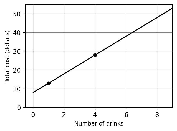
For part 4: \(8 + 5x = 50 \Rightarrow 5x = 42 \Rightarrow x = 8.4\). At 8 drinks the cost is $48; at 9 drinks it would be $53. So one can order up to 8 drinks before the total exceeds $50.
Exercise 19.4 It’s firewood season, and if you don’t own a chainsaw, you might need to rent one. At Taos Tool Rental, customers pay a rental fee and also pay per hour of use for a chainsaw.
- Marcus rents a chainsaw for 3 hours and is charged a total of $35.
- Elena rents a chainsaw for 7 hours and is charged a total of $55.
- Determine the per-hour cost and also the rental fee.
- Make a data table showing the total cost for up to 10 hours.
- Make a plot showing cost on the vertical axis and number of hours on the horizontal axis.
- How many hours can one rent the chainsaw before the total cost exceeds $75?
Solutions
Let \(x\) = number of hours, \(y\) = total cost (dollars).
Rate: \(\dfrac{55 - 35}{7 - 3} = \dfrac{20}{4} = 5\) dollars per hour. Rental fee: \(35 = 5(3) + b \Rightarrow b = 20\).
Equation: \(y = 20 + 5x\).
| \(x\) (hours) | \(y\) (dollars) |
|---|---|
| 0 | 20 |
| 1 | 25 |
| 2 | 30 |
| 3 | 35 |
| 4 | 40 |
| 5 | 45 |
| 6 | 50 |
| 7 | 55 |
| 8 | 60 |
| 9 | 65 |
| 10 | 70 |
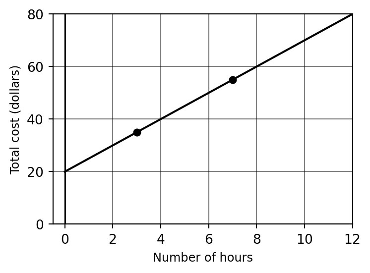
For part 4: \(20 + 5x = 75 \Rightarrow 5x = 55 \Rightarrow x = 11\) hours.