27 Practice with exponential models
27.1 Exponential scenarios
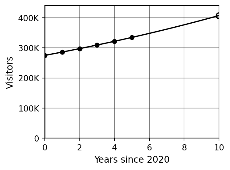
Example 27.1 (Activity: Taos Ski Valley visitors) The Taos Ski Valley reports that the number of visitors has been growing at a steady rate of 4% per year. In 2020, the ski valley welcomed 275,000 visitors.
- Make a data table showing the number of visitors for the five years following 2020.
- Construct a formula for the number of visitors in terms of years since 2020.
- Sketch a plot of your model.
- According to your model, how many visitors will the ski valley welcome in 2030?
Solutions
\(A = 275000\), \(r = 0.04\), \(R = 1.04\), \(x =\) years since 2020, \(y =\) number of visitors.
| Year (\(x\)) | Visitors (\(y\)) |
|---|---|
| 0 (2020) | 275,000 |
| 1 (2021) | 286,000 |
| 2 (2022) | 297,440 |
| 3 (2023) | 309,338 |
| 4 (2024) | 321,711 |
| 5 (2025) | 334,580 |
Formula: \(y = 275000 \cdot (1.04)^x\).
2030 (\(x = 10\)): \(y = 275000 \cdot (1.04)^{10} \approx 275000 \cdot 1.4802 \approx 407{,}059\) visitors.
Filled circles = data table values; hollow circle = 2030 prediction.
Example 27.2 (Activity: Alfalfa hay spoilage) A rancher starts winter with 120 bales of alfalfa hay. Unfortunately, 40% of the remaining hay is lost to spoilage each month.
- Make a data table showing the number of bales remaining each month for 5 months.
- Construct a formula for the number of bales in terms of months.
- Sketch a plot of your model.
- How many bales remain after 8 months? Is that a practical amount?
Solutions
\(A = 120\), \(r = 0.40\) (spoilage rate), \(R = 1 - 0.40 = 0.60\), \(x =\) months, \(y =\) bales remaining.
| Month (\(x\)) | Bales (\(y\)) |
|---|---|
| 0 | 120.0 |
| 1 | 72.0 |
| 2 | 43.2 |
| 3 | 25.9 |
| 4 | 15.6 |
| 5 | 9.3 |
Formula: \(y = 120 \cdot (0.60)^x\).
After 8 months: \(y = 120 \cdot (0.60)^8 \approx 120 \cdot 0.01680 \approx 2.0\) bales. At that point the rancher has essentially run out of usable hay.
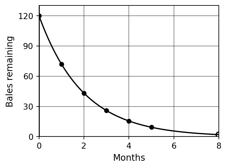
Filled circles = data table values; hollow circle = month 8 prediction.
Example 27.3 (Activity: Sourdough starter) A bread baker starts a sourdough culture with 10 grams of wild yeast. Under ideal conditions, the culture grows at a rate of 20% per day.
- Make a data table showing the amount of culture each day for one week.
- Construct a formula for the amount of culture in terms of days.
- Sketch a plot of your model.
- How much starter does the baker have after two weeks?
Solutions
\(A = 10\), \(r = 0.20\), \(R = 1.20\), \(x =\) days, \(y =\) grams of culture.
| Day (\(x\)) | Culture (\(y\), grams) |
|---|---|
| 0 | 10.0 |
| 1 | 12.0 |
| 2 | 14.4 |
| 3 | 17.3 |
| 4 | 20.7 |
| 5 | 24.9 |
| 6 | 29.9 |
| 7 | 35.8 |
Formula: \(y = 10 \cdot (1.20)^x\).
After two weeks (\(x = 14\)): \(y = 10 \cdot (1.20)^{14} \approx 10 \cdot 12.84 \approx 128.4\) grams.
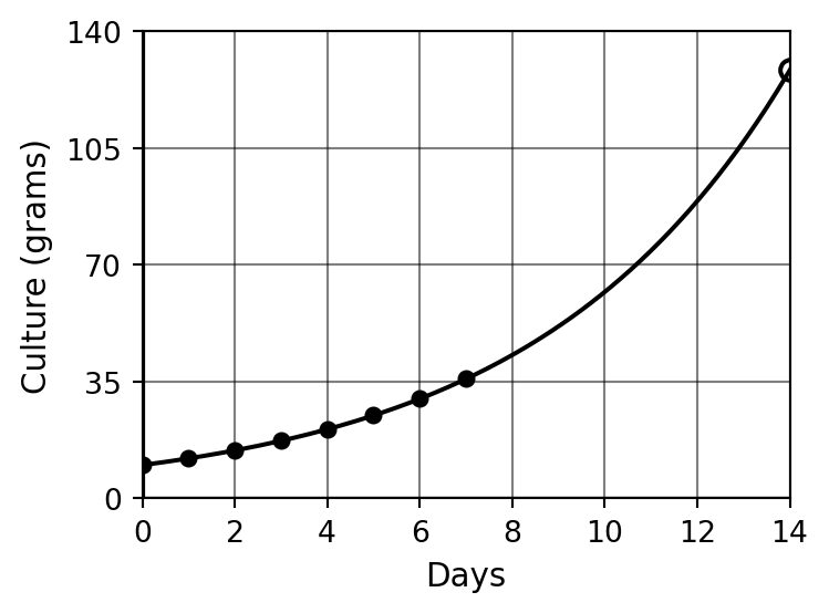
Filled circles = data table values; hollow circle = day 14 prediction.
Example 27.4 (Activity: Quarterly investment) A UNM-Taos employee invests $1,500 in a retirement fund earning 6% annually, compounded quarterly.
- Make a data table showing the value of the investment each quarter for the first 4 quarters.
- Construct a formula for the value in terms of quarters.
- Sketch a plot of your model.
- What will the investment be worth after 10 years?
Solutions
\(A = 1500\), \(r = 0.06\), \(N = 4\) quarters per year, \(R = 1 + \dfrac{0.06}{4} = 1.015\), \(x =\) quarters.
| Quarter (\(x\)) | Value (\(y\)) |
|---|---|
| 0 | $1,500.00 |
| 1 | $1,522.50 |
| 2 | $1,545.34 |
| 3 | $1,568.52 |
| 4 | $1,592.05 |
Formula: \(y = 1500 \cdot (1.015)^x\).
After 10 years = 40 quarters: \(y = 1500 \cdot (1.015)^{40} \approx 1500 \cdot 1.8140 \approx \$2{,}721\).

Filled circles = data table values; hollow circle = 10-year prediction.
27.2 Interpreting exponential plots
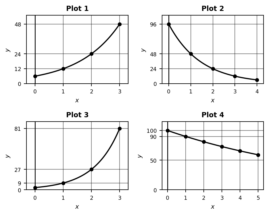
Example 27.5 (Activity: Reading exponential plots) Each plot below shows an exponential model \(y = A \cdot R^x\). Two points on each curve are labeled.
For each plot, determine the values of \(A\) and \(R\), and write the formula.
For each plot, fill in the table below.
| \(A\) | \(R\) | Formula | |
|---|---|---|---|
| Plot 1 | |||
| Plot 2 | |||
| Plot 3 | |||
| Plot 4 |
Which plots show increasing exponential models? Which show decreasing?
Solutions
| \(A\) | \(R\) | Formula | |
|---|---|---|---|
| Plot 1 | 6 | 2 | \(y = 6 \cdot 2^x\) |
| Plot 2 | 96 | \(\frac{1}{2}\) | \(y = 96 \cdot \left(\frac{1}{2}\right)^x\) |
| Plot 3 | 3 | 3 | \(y = 3 \cdot 3^x\) |
| Plot 4 | 100 | 0.9 | \(y = 100 \cdot (0.9)^x\) |
In each case: \(R = \dfrac{\text{value at } x=1}{\text{value at } x=0}\). For example, Plot 1: \(R = \dfrac{12}{6} = 2\).
Increasing: Plots 1 and 3 (\(R > 1\)). Decreasing: Plots 2 and 4 (\(0 < R < 1\)).
27.3 Interpreting exponential formulas
Example 27.6 (Activity: Annual growth model) Consider the exponential model \[ y = 200 \cdot (1.15)^x, \] where \(x\) is measured in years.
- What is the starting amount \(A\)?
- What is the multiplier \(R\)? What is the annual percent growth rate \(r\)?
- Is this model increasing or decreasing? How can you tell from \(R\)?
- What will the amount be after 10 years?
Solutions
\(A = 200\).
\(R = 1.15\). Since \(R = 1 + r\), we get \(r = 0.15\), i.e., a 15% annual growth rate.
The model is increasing because \(R = 1.15 > 1\).
After 10 years: \(y = 200 \cdot (1.15)^{10} \approx 200 \cdot 4.046 \approx 809\).
Example 27.7 (Activity: Monthly decay model) Consider the exponential model \[ y = 1200 \cdot (0.82)^x, \] where \(x\) is measured in months.
- What is the starting amount \(A\)?
- What is the multiplier \(R\)? What is the monthly percent decrease rate \(r\)?
- Is this model increasing or decreasing? How can you tell from \(R\)?
- What will the amount be after 6 months?
Solutions
\(A = 1200\).
\(R = 0.82\). Since \(R = 1 - r\), we get \(r = 1 - 0.82 = 0.18\), i.e., an 18% monthly decrease rate.
The model is decreasing because \(R = 0.82 < 1\).
After 6 months: \(y = 1200 \cdot (0.82)^6 \approx 1200 \cdot 0.3040 \approx 365\).
Example 27.8 (Activity: Quarterly compounding model) Consider the exponential model \[ y = 3500 \cdot \left(1 + \frac{0.045}{4}\right)^x, \] where \(x\) is measured in quarters.
- What is the starting amount \(A\)?
- What is the annual rate \(r\)? What is \(N\)? How often is the rate compounded?
- What is the multiplier \(R\)?
- What will the amount be after 5 years?
Solutions
\(A = 3500\).
\(r = 0.045\) (4.5% annual rate), \(N = 4\) (compounded quarterly, i.e., four times per year).
\(R = 1 + \dfrac{0.045}{4} = 1 + 0.01125 = 1.01125\).
After 5 years = 20 quarters: \(y = 3500 \cdot (1.01125)^{20} \approx 3500 \cdot 1.2507 \approx \$4{,}378\).
27.4 Reading exponential models from data tables
Example 27.9 (Activity: Which tables are exponential?) Each table below shows the data table of some model. For each table, determine whether the model is linear, exponential, or neither. For any table that is exponential, identify \(A\) and \(R\) and write the formula.
Table A
| \(x\) | \(y\) |
|---|---|
| 0 | 4 |
| 1 | 12 |
| 2 | 36 |
| 3 | 108 |
Table B
| \(x\) | \(y\) |
|---|---|
| 0 | 100 |
| 1 | 85 |
| 2 | 70 |
| 3 | 55 |
Table C
| \(x\) | \(y\) |
|---|---|
| 0 | 200 |
| 1 | 160 |
| 2 | 128 |
| 3 | 102.4 |
Solutions
Table A: Ratios: \(\dfrac{12}{4} = 3\), \(\dfrac{36}{12} = 3\), \(\dfrac{108}{36} = 3\). Constant ratio — exponential. \(A = 4\), \(R = 3\). Formula: \(y = 4 \cdot 3^x\).
Table B: Differences: \(85 - 100 = -15\), \(70 - 85 = -15\), \(55 - 70 = -15\). Constant difference — linear. (Not exponential.)
Table C: Ratios: \(\dfrac{160}{200} = 0.8\), \(\dfrac{128}{160} = 0.8\), \(\dfrac{102.4}{128} = 0.8\). Constant ratio — exponential. \(A = 200\), \(R = 0.8\). Formula: \(y = 200 \cdot (0.8)^x\).
Example 27.10 (Activity: Which tables are exponential?) Each table below shows the data table of some model. For each table, determine whether the model is linear, exponential, or neither. For any table that is exponential, identify \(A\) and \(R\), write the formula, and use the formula to predict the value at \(x = 5\).
Table A
| \(x\) | \(y\) |
|---|---|
| 0 | 6 |
| 1 | 18 |
| 2 | 54 |
| 3 | 162 |
Table B
| \(x\) | \(y\) |
|---|---|
| 0 | 500 |
| 1 | 400 |
| 2 | 320 |
| 3 | 256 |
Table C
| \(x\) | \(y\) |
|---|---|
| 0 | 10 |
| 1 | 25 |
| 2 | 45 |
| 3 | 70 |
Solutions
Table A: Ratios: \(\dfrac{18}{6} = 3\), \(\dfrac{54}{18} = 3\), \(\dfrac{162}{54} = 3\). Exponential. \(A = 6\), \(R = 3\). Formula: \(y = 6 \cdot 3^x\). At \(x = 5\): \(y = 6 \cdot 3^5 = 6 \cdot 243 = 1{,}458\).
Table B: Ratios: \(\dfrac{400}{500} = 0.8\), \(\dfrac{320}{400} = 0.8\), \(\dfrac{256}{320} = 0.8\). Exponential. \(A = 500\), \(R = 0.8\). Formula: \(y = 500 \cdot (0.8)^x\). At \(x = 5\): \(y = 500 \cdot (0.8)^5 \approx 163.8\).
Table C: Differences: \(25 - 10 = 15\), \(45 - 25 = 20\), \(70 - 45 = 25\). Ratios: \(\dfrac{25}{10} = 2.5\), \(\dfrac{45}{25} = 1.8\), \(\dfrac{70}{45} \approx 1.56\). Neither constant differences nor constant ratios — neither linear nor exponential.