14 Data plots
Data plots are a way to visualize information that appears in a data table. Let’s introduce data plots with the following simple example.
14.1 Jordan goes for a walk
On Saturday mornings, Jordan goes for a long walk. His walking speed is \(3\) miles per hour.
Let’s explore this scenario using these variables:
- \(x\) is the time walked (in hours)
- \(y\) is the distance walked (in miles)
Description via data table
The following table gives a list of values for \(x\). Fill in the missing values for \(y\).
| \(x=\) time | \(y=\) distance |
|---|---|
| 0 | 0 |
| 1 | 3 |
| 2 | 6 |
| 3 | |
| 4 |
Description via plot
We visually represent the relationship between time and distance using a plot in the Cartesian plane. The plot is organized in the following way:
- We make a horizonal number line that represents values of \(x\).
- We make a vertical number line that represents values of \(y\).
Each row in our table of values represents a pair of values for \(x\) and \(y\). Using the horizontal and vertical number lines, we mark a corresponding point in the plot. In the following graphic, the first three data points are indicated.
Example 14.1 (Activity: adding data points) Add the remaining two data points from the table of values to the plot above.
Solutions
The remaining points are \((3, 9)\) and \((4, 12)\).
14.2 Plotting and the Cartesian Plane
In the motivating example above, we introduced the idea of plotting using the Cartesian plane. Let’s explore the Cartesian plane in more detail.
Axes and Variables
The horizontal and vertical number lines are called axes.
While any variable name can be used to describe the axes, there are standard default settings:
- The default setting for the horizontal axis is the variable \(x\).
- The default setting for the vertical axis is the variable \(y\).
The place where the two axes meet is called the origin, and corresponds to both variables being equal to zero.
Ordered pair notation
When identifying a location in the plane, we can specify the \(x\) and \(y\) values individually. We call these values coordinates. For example, location \(A\) in the graphic below has coordinates \(x=2\) and \(y=3\).
We use ordered pairs of numbers as a shortcut notation. Thus we can simply say that location \(A\) has coordinates \((2,3)\). Always we list the horizontal value first, followed by the vertical value.
Example 14.2 (Activity: reading coordinates) Use the graphic above to identify the coordinates of each point. \[ \begin{aligned} A &= (2,3) &\qquad B &=\qquad &\qquad C &= \qquad &\qquad D &= \qquad \\[10pt] E &=\qquad &\qquad F &=\qquad &\qquad G &=\qquad &\qquad H&= \qquad \end{aligned} \]
Solutions
\(A=(2,3)\), \(B=(-3,4)\), \(C=(4,-2)\), \(D=(-2,-3)\), \(E=(0,2)\), \(F=(3,0)\), \(G=(-4,-1)\), \(H=(1,-4)\).
14.3 Examples from Chapter 13
We can make plots of the tables constructed in Chapter 13.
Example 14.3 (Activity: plot Mora County population) Construct a plot showing the data from the table in Example 13.1.
Before you start drawing the plot, think carefully about plotting scale — what are the smallest and largest values you will need for both vertical and horizontal parts of the plot?

Solutions
Axis scales: horizontal (\(x\) = year) from 1975 to 2025; vertical (\(y\) = population) from 4,000 to 5,500.
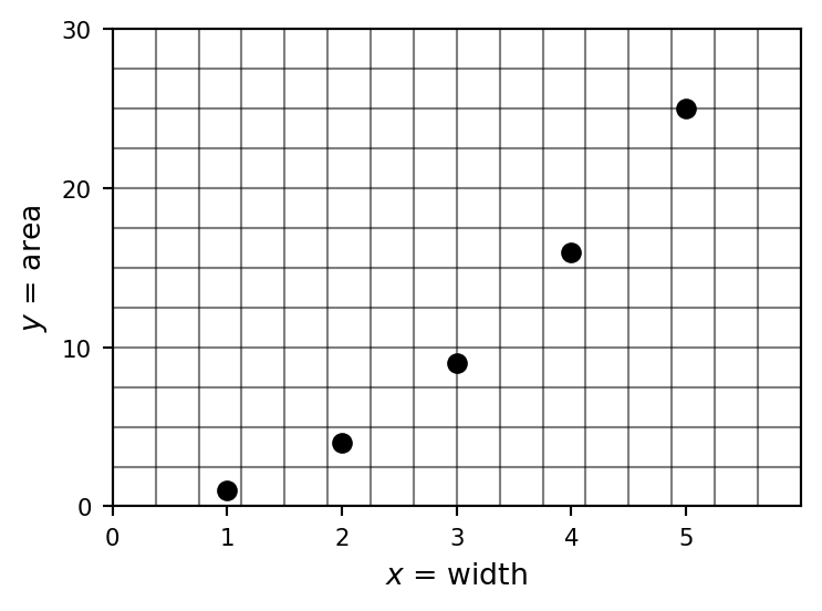
Example 14.4 (Activity: plot square area) Construct a plot showing the data from the table in Example 13.2.
Before you start drawing the plot, think carefully about plotting scale — what are the smallest and largest values you will need for both vertical and horizontal parts of the plot?

Solutions
Axis scales: horizontal (\(x\) = width) from 0 to 6; vertical (\(y\) = area) from 0 to 30.
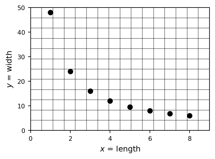
Example 14.5 (Activity: plot rectangle dimensions) Construct a plot showing the data from the table in Example 13.3.
Before you start drawing the plot, think carefully about plotting scale — what are the smallest and largest values you will need for both vertical and horizontal parts of the plot?

Solutions
Axis scales: horizontal (\(x\) = length) from 0 to 9; vertical (\(y\) = width) from 0 to 50.
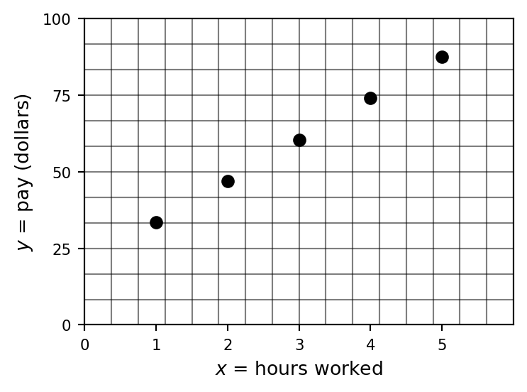
Example 14.6 (Activity: plot coffee wages) Construct a plot showing the data from the table in Example 13.4.
Before you start drawing the plot, think carefully about plotting scale — what are the smallest and largest values you will need for both vertical and horizontal parts of the plot?

Solutions
Axis scales: horizontal (\(x\) = hours worked) from 0 to 6; vertical (\(y\) = pay) from 0 to 100.
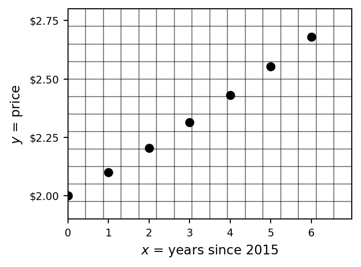
Example 14.7 (Activity: plot coffee price) Construct a plot showing the data from the table in Example 13.5.
Before you start drawing the plot, think carefully about plotting scale — what are the smallest and largest values you will need for both vertical and horizontal parts of the plot?
Solutions
Axis scales: horizontal (\(x\) = years since 2015) from 0 to 7; vertical (\(y\) = price) from $1.90 to $2.80.
14.4 Homework exercises
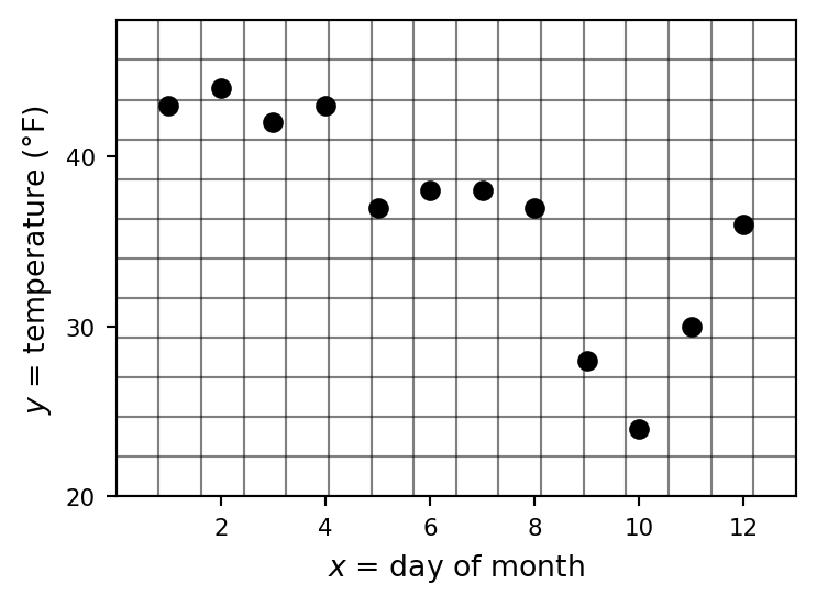
Exercise 14.1 Construct a plot corresponding to the data table you made in Exercise 13.1.

Solutions
Axis scales: horizontal (\(x\) = day) from 0 to 13; vertical (\(y\) = temperature °F) from 20 to 48.
Exercise 14.2 Construct a plot corresponding to the data table you made in Exercise 13.2.

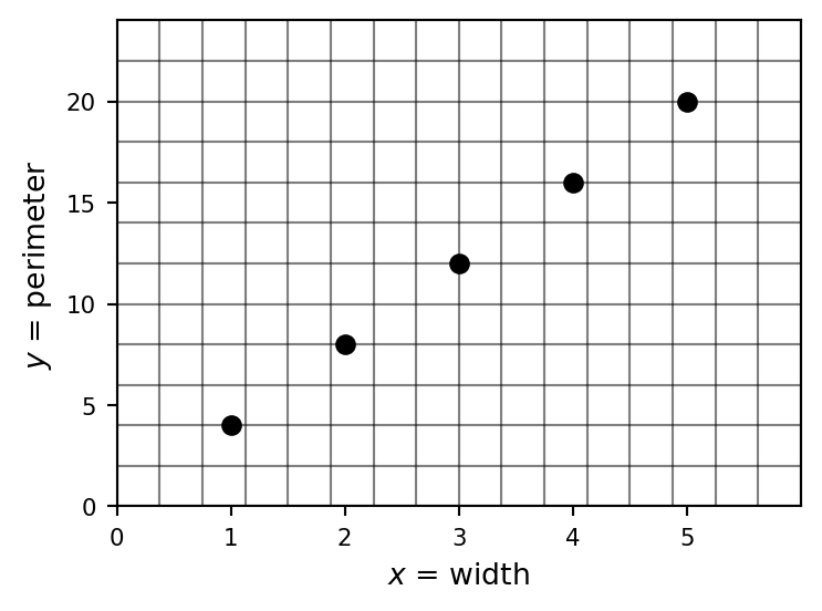
Exercise 14.3 Construct a plot corresponding to the data table you made in Exercise 13.3.

Solutions
Axis scales: horizontal (\(x\) = width) from 0 to 6; vertical (\(y\) = perimeter) from 0 to 24.
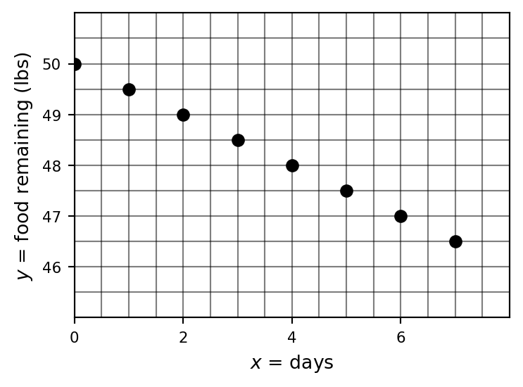
Exercise 14.4 Construct a plot corresponding to the data table you made in Exercise 13.4.

Solutions
Axis scales: horizontal (\(x\) = days) from 0 to 8; vertical (\(y\) = food remaining, lbs) from 45 to 51.
Exercise 14.5 Construct a plot corresponding to the data table you made in Exercise 13.5.

Solutions
Axis scales: horizontal (\(x\) = years) from 0 to 6; vertical (\(y\) = value) from $14,000 to $21,000.