23 The basic exponential model
The goal of this section is to introduce a type of nonlinear model called a basic exponential model. We start with three motivating examples.
Example 23.1 (Activity: Comparing two payment plans) Winners of the Taos County Xtreme Lottery receive an initial payment when they win, and then receive additional payments over a 30 week time period. They have a choice about how they want to receive their payments:
Option 1 is to receive an initial $10,000 and then receive a $10,000 check each week for the next 30 weeks.
Option 2 is to receive an initial payment of 1 penny ($0.01), and then have the payment double each week during the 30 week time period.
Complete the data table below.
| Week | Option 1 Payment | Option 2 Payment |
|---|---|---|
| 0 | $10,000 | $0.01 |
| 1 | $10,000 | \(0.01 \cdot 2 = \$0.02\) |
| 2 | $10,000 | \(0.01\cdot 2\cdot 2 = \$0.04\) |
| 3 | ||
| 4 | ||
| 5 | ||
| \(\phantom{\dfrac{1}{2}}\) | ||
| \(\phantom{\dfrac{1}{2}}\) |
Using the variables
- \(x\) is the number of weeks,
- \(y\) is the Option 2 payment (in dollars),
the formula for Option 2 is \[ y = \underline{\hspace{2in}} \]
Using your formula, what is the Option 2 payment in Week 30?
How does the Option 2 payment in Week 30 compare to the total of all payments in Option 1?
In what week does the Option 2 payment first exceed the Option 1 payment? (Hint: experiment with your formula.)
Solutions
The Option 2 payment doubles each week:
| Week | Option 1 Payment | Option 2 Payment |
|---|---|---|
| 0 | $10,000 | $0.01 |
| 1 | $10,000 | $0.02 |
| 2 | $10,000 | $0.04 |
| 3 | $10,000 | $0.08 |
| 4 | $10,000 | $0.16 |
| 5 | $10,000 | $0.32 |
The formula is \(y = 0.01 \cdot 2^x\).
Week 30 payment: \(y = 0.01 \cdot 2^{30} = 0.01 \cdot 1{,}073{,}741{,}824 \approx \$10{,}737{,}418\).
Comparison: Option 1 pays 31 payments of $10,000 each for a total of $310,000. The single Week 30 Option 2 payment exceeds $10 million — far more than all of Option 1 combined.
When Option 2 first exceeds Option 1: We need \(0.01 \cdot 2^x > 10{,}000\). Checking: \(2^{19} = 524{,}288\) gives $5,243, and \(2^{20} = 1{,}048{,}576\) gives $10,486. Option 2 first exceeds Option 1 in Week 20.
Example 23.2 (Activity: Mayor Dan’s PSA) Mayor Dan records a short public service announcement video and posts it to all the socials. Initially, the video gets only 10 views. But the video spreads! Each day, the number of views is 5 times the number of the previous day.
- Make a data table showing the number of views each day for the first 5 days.
- Plot your data on the following axes.
- Using the variables
- \(x\) is the number of days since posting,
- \(y\) is the number of views,
construct a formula for the number of views each day.
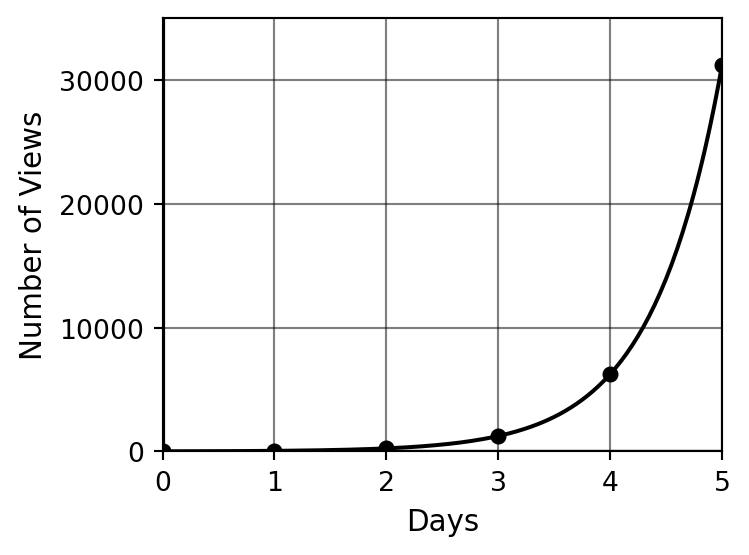
Solutions
| Day (\(x\)) | Views (\(y\)) |
|---|---|
| 0 | 10 |
| 1 | 50 |
| 2 | 250 |
| 3 | 1,250 |
| 4 | 6,250 |
| 5 | 31,250 |
The formula is \(y = 10 \cdot 5^x\).
Example 23.3 (Activity: Diagnostic iodine) Iodine-123 is used for medical imaging, because it emits gamma rays as it decays away. The rate of decay for Iodine-123 is such that after 1 day, roughly 75% has decayed away, leaving only 25% of what was there the previous day. A lab starts the week with 48 grams of Iodine-123.
- Make a data table showing the amount of Iodine-123 that remains over the course of 7 days.
- Plot your data on the following axes.
- Using the variables
- \(x\) is the number of days since the start of the week,
- \(y\) is the amount of Iodine-123 (in grams),
construct a formula for the amount remaining each day.
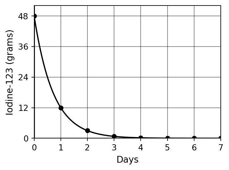
Solutions
| Day (\(x\)) | Iodine-123 (\(y\), grams) |
|---|---|
| 0 | 48 |
| 1 | 12 |
| 2 | 3 |
| 3 | 0.75 |
| 4 | 0.188 |
| 5 | 0.047 |
| 6 | 0.012 |
| 7 | 0.003 |
The formula is \(y = 48 \cdot \left(\dfrac{1}{4}\right)^x\).
23.1 Discussion: features of an exponential model
All three motivating examples above involve exponential models. The word exponential is used because the formulas have the input variable \(x\) located in the exponent. Let’s identify the common features of these examples.
- What do the three scenarios have in common?
- What do the data tables in the three examples have in common?
- What do the formulas in the three examples have in common?
- The plots of the three examples look very different. What types of behaviors can we expect from exponential models?
Solutions
Scenarios: In each example, the quantity changes by a constant multiplier during each time period — doubling, multiplying by 5, or multiplying by \(\frac{1}{4}\) — rather than by a constant addition as in linear models.
Data tables: The ratio between any two consecutive output values is constant. Dividing any output value by the previous one gives the same number each time.
Formulas: Each formula has the structure (starting amount) \(\cdot\) (constant ratio)\(^x\), with the variable \(x\) appearing in the exponent.
Plots: Exponential models can grow rapidly (lottery, Mayor Dan) or decay toward zero (iodine). In all cases the graph is a curve, not a straight line.