24 The exponential model framework
In the previous section we explored examples of exponential models and noted their common features. We now develop a general framework for describing and working with exponential models.
24.1 Parameters of the exponential model
Exponential models are determined by two numbers:
- \(A =\) the starting amount (also called the initial value)
- \(R =\) the ratio (also called the multiplier) by which the amount changes in one unit of time
24.2 Discussion: Where do \(A\) and \(R\) appear?
In each example, \(A\) is the starting value. Where does \(A\) appear in the data table? Where does \(A\) appear in the plot?
In each example, \(R\) is the constant multiplier. Where does \(R\) appear in the data table? Where does \(R\) appear in the plot?
Solutions
\(A\) in the data table: \(A\) is the output value when \(x = 0\), i.e., the first entry in the output column.
\(A\) in the plot: \(A\) is the \(y\)-intercept — the point where the curve crosses the vertical axis.
\(R\) in the data table: \(R\) is the constant ratio between any two consecutive output values. Dividing any output value by the one before it always gives \(R\).
\(R\) in the plot: \(R\) controls the shape of the curve. A large \(R > 1\) produces a steeply rising curve; a small \(0 < R < 1\) produces a curve that drops sharply toward zero.
24.3 General formula
The general formula for the basic exponential model is \[ y = A \cdot R^x. \]
Take a moment to verify that this formula matches the Mayor Dan and iodine examples from the previous section.
24.4 Exponential increase and decrease
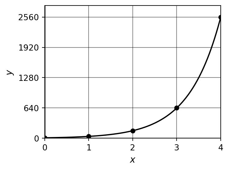
Example 24.3 (Activity: An increasing exponential model) Consider the exponential model \(y = 10 \cdot 4^x\).
What is the starting amount for this model? What is the ratio?
Make a data table for this model.
Sketch the plot for this model.
What do you expect to happen to \(y\) when \(x\) is very large?
Solutions
| \(x\) | \(y = 10 \cdot 4^x\) |
|---|---|
| 0 | 10 |
| 1 | 40 |
| 2 | 160 |
| 3 | 640 |
| 4 | 2,560 |
As \(x\) grows large, \(y\) grows without bound toward \(+\infty\).
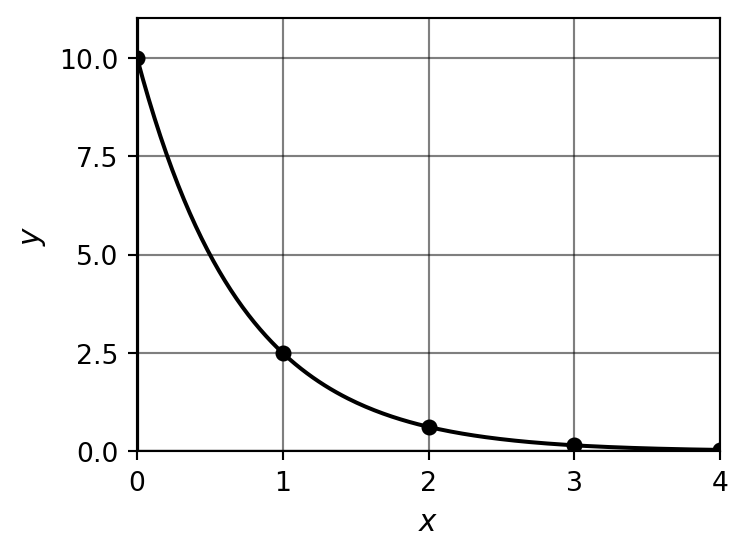
Example 24.4 (Activity: A decreasing exponential model) Consider the exponential model \(y = 10 \cdot \left(\dfrac{1}{4}\right)^x\).
What is the starting amount for this model? What is the ratio?
Make a data table for this model.
Sketch the plot for this model.
What do you expect to happen to \(y\) when \(x\) is very large?
Solutions
| \(x\) | \(y = 10 \cdot \left(\dfrac{1}{4}\right)^x\) |
|---|---|
| 0 | 10 |
| 1 | 2.5 |
| 2 | 0.625 |
| 3 | 0.156 |
| 4 | 0.039 |
As \(x\) grows large, \(y\) decreases toward \(0\) but never actually reaches \(0\).
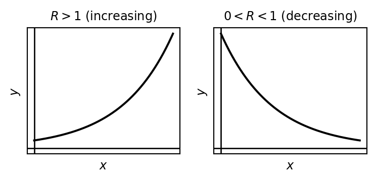
24.5 Discussion: increasing and decreasing models
Some exponential models are increasing and some are decreasing. How can we tell which is which by looking at the value of \(R\)?
Sketch the plot of a typical increasing exponential model.
Sketch the plot of a typical decreasing exponential model.
Solutions
If \(R > 1\), then each output value is larger than the previous one, so the model is increasing.
If \(0 < R < 1\), then each output value is smaller than the previous one, so the model is decreasing.
The line \(y = 0\) is a horizontal asymptote for decreasing models: the values approach zero but never reach it.
24.6 Reading exponential models from data tables
So far we have built exponential models starting from real-world scenarios. We can also move in the other direction: given a data table, determine whether the model is exponential and, if so, identify \(A\) and \(R\).
Example 24.5 (Activity: Reading a data table) The following data table shows values of a model \(y = f(x)\).
| \(x\) | \(y\) |
|---|---|
| 0 | 5 |
| 1 | 15 |
| 2 | 45 |
| 3 | 135 |
| 4 | 405 |
Compute the ratio of each consecutive pair of output values. Is the ratio constant?
Is this model linear, exponential, or neither? Explain.
Identify \(A\) and \(R\), and write the formula \(y = A \cdot R^x\).
Solutions
Ratios: \(\dfrac{15}{5} = 3\), \(\dfrac{45}{15} = 3\), \(\dfrac{135}{45} = 3\), \(\dfrac{405}{135} = 3\). The ratio is constant, so this is an exponential model with \(R = 3\).
\(A = 5\) (the output when \(x = 0\)).
Formula: \(y = 5 \cdot 3^x\).
24.7 Homework exercises
Exercise 24.1 A single yeast cell floats through the air and lands in a bowl of water and flour. Assume that yeast cells divide every minute.
- Make a data table showing the number of yeast cells each minute for the first 8 minutes.
- Explain why a basic exponential model is appropriate for this scenario.
- Construct a plot of the data in your table.
- Construct an equation that describes this scenario.
- Use your equation to predict how many yeast cells there will be after 1 hour. Then predict how many there will be after 1 day.
Solutions
| Minute (\(x\)) | Yeast cells (\(y\)) |
|---|---|
| 0 | 1 |
| 1 | 2 |
| 2 | 4 |
| 3 | 8 |
| 4 | 16 |
| 5 | 32 |
| 6 | 64 |
| 7 | 128 |
| 8 | 256 |
This is exponential because the number of cells doubles every minute — the ratio between consecutive values is the constant \(R = 2\).
Formula: \(y = 2^x\) (with \(A = 1\), \(R = 2\)).
After 1 hour (\(x = 60\)): \(y = 2^{60} \approx 1.15 \times 10^{18}\) cells.
After 1 day (\(x = 1440\)): \(y = 2^{1440}\), an astronomically large number.
Exercise 24.2 Wintertime is pothole season in Taos County, as the freeze/thaw cycle causes the roads to wear faster. At the beginning of the year, there are only 2 potholes on Paseo del Pueblo Sur. Every week, the number of potholes is three times larger than the previous week.
- Make a data table showing the number of potholes during the first 8 weeks of winter.
- Construct a plot of your data.
- Build an exponential formula for the number of potholes in terms of the number of weeks.
Solutions
| Week (\(x\)) | Potholes (\(y\)) |
|---|---|
| 0 | 2 |
| 1 | 6 |
| 2 | 18 |
| 3 | 54 |
| 4 | 162 |
| 5 | 486 |
| 6 | 1,458 |
| 7 | 4,374 |
| 8 | 13,122 |
Formula: \(y = 2 \cdot 3^x\) (with \(A = 2\), \(R = 3\)).
Exercise 24.3 When dropped, the Amazing Bouncy Ball of Antonito bounces back up to half the height from which it was dropped. This continues for each bounce. Suppose the ball is dropped from the roof of the STEM building at a height of 24 feet.
- Make a data table giving the height of the ball in terms of the number of bounces.
- Make a plot of the data in your table.
- Construct a formula for the height in terms of the number of bounces.
- How high will the ball bounce on the 10th bounce?
Solutions
| Bounce (\(x\)) | Height (\(y\), feet) |
|---|---|
| 0 | 24 |
| 1 | 12 |
| 2 | 6 |
| 3 | 3 |
| 4 | 1.5 |
| 5 | 0.75 |
Formula: \(y = 24 \cdot \left(\dfrac{1}{2}\right)^x\) (with \(A = 24\), \(R = \dfrac{1}{2}\)).
10th bounce: \(y = 24 \cdot \left(\dfrac{1}{2}\right)^{10} = \dfrac{24}{1024} \approx 0.023\) feet (less than a third of an inch).
Exercise 24.4 On a cold winter day in Taos, a math teacher accidentally leaves their coffee cup on the railing of their front porch. When first left behind, the coffee was 80 degrees Celsius. Each minute, the coffee is nine-tenths as warm as it was the previous minute.
- Make a data table giving the temperature of the coffee each minute for a period of 5 minutes.
- Make a plot of the data in your table.
- Construct a formula for the temperature of the coffee in terms of minutes.
- What will the temperature be after 15 minutes, when the math teacher goes to fetch it?
Solutions
| Minute (\(x\)) | Temperature (\(y\), °C) |
|---|---|
| 0 | 80.0 |
| 1 | 72.0 |
| 2 | 64.8 |
| 3 | 58.3 |
| 4 | 52.5 |
| 5 | 47.2 |
Formula: \(y = 80 \cdot (0.9)^x\) (with \(A = 80\), \(R = 0.9\)).
After 15 minutes: \(y = 80 \cdot (0.9)^{15} \approx 80 \cdot 0.206 \approx 16.5\)°C (about 62°F — quite cold).
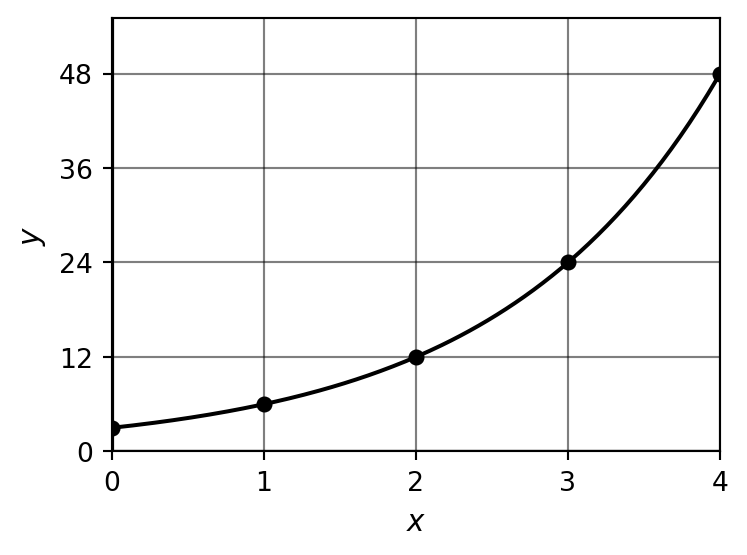
Exercise 24.5 Make a data table and a plot for the basic exponential model \(y = 3\cdot 2^x\).
Solutions
| \(x\) | \(y = 3 \cdot 2^x\) |
|---|---|
| 0 | 3 |
| 1 | 6 |
| 2 | 12 |
| 3 | 24 |
| 4 | 48 |
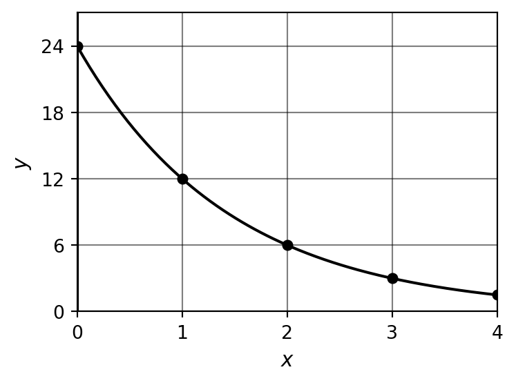
Exercise 24.6 Make a data table and a plot for the basic exponential model \(y = 24\cdot \left(\dfrac{1}{2}\right)^x\).
Solutions
| \(x\) | \(y = 24 \cdot \left(\dfrac{1}{2}\right)^x\) |
|---|---|
| 0 | 24 |
| 1 | 12 |
| 2 | 6 |
| 3 | 3 |
| 4 | 1.5 |
Exercise 24.7 Consider the following scenarios. Determine whether a linear model or a basic exponential model would be more appropriate for each.
- Each day, five soda cans are added to the recycle bin.
- Each century, half of the radioactive material decays away.
- Each semester, there are an additional 150 students attending UNM-Taos.
- The cost of housing doubles every decade.
- Each year, the price of a bowl of posole goes up by $0.50.
- Each year, the price of a breakfast burrito goes up by 5%.
Solutions
- Soda cans: Linear — the amount increases by a constant addition of 5 each day.
- Radioactive material: Exponential — the amount is multiplied by \(\frac{1}{2}\) each century (\(R = \frac{1}{2}\)).
- UNM-Taos students: Linear — the count increases by a constant addition of 150 each semester.
- Housing cost: Exponential — the cost is multiplied by 2 each decade (\(R = 2\)).
- Posole: Linear — the price increases by a constant addition of $0.50 each year.
- Breakfast burrito: Exponential — the price is multiplied by 1.05 each year (\(R = 1.05\)).
Exercise 24.8 The following data table shows values of a model \(y = f(x)\).
| \(x\) | \(y\) |
|---|---|
| 0 | 80 |
| 1 | 40 |
| 2 | 20 |
| 3 | 10 |
| 4 | 5 |
- Compute the ratio of each consecutive pair of output values to confirm that this is an exponential model.
- Identify \(A\) and \(R\). Use them to write the formula \(y = A \cdot R^x\) that matches the data table.
- Use your formula to predict the value at \(x = 6\).
Solutions
Ratios: \(\dfrac{40}{80} = \dfrac{1}{2}\), \(\dfrac{20}{40} = \dfrac{1}{2}\), \(\dfrac{10}{20} = \dfrac{1}{2}\), \(\dfrac{5}{10} = \dfrac{1}{2}\). The ratio is constant, confirming an exponential model.
\(A = 80\), \(R = \dfrac{1}{2}\). The formula is \(y = 80 \cdot \left(\dfrac{1}{2}\right)^x\).
At \(x = 6\) we have \(y = 80 \cdot \left(\dfrac{1}{2}\right)^6 = 80 \cdot \dfrac{1}{64} = 1.25\).